Antenna Basics

Fundamental Definitions

Antennas are the connecting link between RF signals in an electrical circuit such as a PCB and an electromagnetic wave propagating in the transmission media between the transmitter and the receiver of a wireless link.

In the transmitter, the antenna transforms the electrical signal into an electromagnetic wave by exciting either an electrical or a magnetic field in its immediate surroundings, the near field. Antennas that excite an electrical field are referred to as electrical antennas; antennas exciting a magnetic field are called magnetic antennas correspondingly. The oscillating electrical or magnetic field generates an electromagnetic wave that propagates with the velocity of light c. The speed of light in free space c0 is 300000 km/s. If the wave travels in a dielectric medium with the relative dielectric constant εr, the speed of light is reduced to:

We can calculate the wavelength from the frequency f of the signal and the speed of light c using the formula:

Using common units, the equation:

is often used for the wavelength in free space. If the wave travels in a dielectric medium, for instance in the PCB material, the wavelength has to be divided by the square root of εr. We can distinguish three field regions where the electromagnetic wave develops: reactive near field, radiating near field and far field:

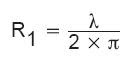
In the reactive near field, reactive field components predominate over the radiated field. This means that any variations in the electrical properties (for electrical antennas) or magnetic properties (for magnetic antennas) have a strong influence on the antenna’s impedance at the antenna feed point. The distance from the antenna to the boundary of the reactive near field region is commonly assumed as:

In the radiating near field the radiated field predominates, the antenna impedance is only slightly influenced by the surrounding media in this region. But the dimensions of the antenna can not be neglected with respect to the distance from the antenna. This means that the angular distribution of the radiation pattern is dependent on the distance. For measurements of the radiation pattern, the distance from the antenna should be larger than the radiating near field boundary, otherwise the measured pattern will be different from that under real life conditions. The diameter of the radiating near field is

with D as the largest dimension of the antenna.

For distances larger than R2, the radiation pattern is independent on the distance; we are in the far field region. The distance between transmitter and receiver antennas in a practical application is usually in this region.

In the receiver, the antenna gathers energy from the electromagnetic wave and transforms it into an electrical voltage and current in the electrical circuit. For better comprehension, the antenna parameters are often explained on a transmit antenna, but in most cases, if no nonlinear ferrites are involved, the characteristics of an antenna are identical in receive and transmit modes.

Antenna Characteristics

Polarization describes the trace that the tip of the electrical field vector builds during the propagation of the wave. In the far field, we can consider the electromagnetic wave as a plane wave. In a plane electromagnetic wave, the electrical and the magnetic field vectors are orthogonal to the direction of propagation and also orthogonal to each other. In the general case, the tip of the electrical field vector moves along an elliptical helix, giving an elliptical polarization. The wave is called right-hand polarized if the tip of the electrical field vector turns clockwise while propagating; otherwise it is left-hand polarized.

If the two axis of the ellipse have the same magnitude, the polarization is called circular. If one of the two axis of the ellipse becomes zero, we have linear polarization, vertical if the electrical field vector oscillates perpendicularly to ground, horizontal if its direction of oscillation is parallel to the ground plane.

A transmission system has the best performance (ideal case) when the polarization of the transmitter and the receiver antenna are identical to each other. Circular polarization on one end and linear polarization on the other gives 3-dB loss compared to the ideal case. If both antennas are linearly polarized but 90° turned to each other, theoretically no power is received. The same phenomenon happens if one antenna is right-hand circularly polarized and the other one left-hand circularly polarized.

In an indoor environment, reflections in the transmission path may change the polarization, which makes the polarization of the received wave difficult to predict. If one of the antennas is portable, we have to make sure that it works in any position. Circular polarization at one end and linear polarization at the other end results in a principal loss of 3 dB, but avoids the case of a total blackout, where no power is received.

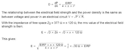
For the description of the radiated power and the gain of the antenna often the concept of the isotropic radiator is used. The isotropic radiator is a hypothetical antenna, which radiates the supplied RF power equally in all directions. The power density at a distance r from the isotropic radiator is therefore the supplied power divided by the area of a sphere with the radius r.

If we measure the power density in some distance from a device under test, the effective isotropic radiated power, EIRP, is the power which we would have to supply to an isotropic radiator in order to get the same power density in the same distance. The EIRP describes the power radiation capability of a device including its antenna.

From the EIRP, we can calculate the electrical field strength at a given distance from the radiator, which is specified in some government or regional regulations. The density of the radiated power D (in W/m2) measured in the distance r from an isotropic radiator radiating the total power EIRP is the radiated power divided by the surface area of the sphere with the radius r:

As opposed to the (only hypothetical) isotropic radiator, real antennas exhibit more or less distinct directional radiation characteristics.

The radiation pattern of an antenna is the normalized polar plot of the radiated power density, measured at a constant distance from the antenna in a horizontal or vertical plane.

The isotropic gain Giso of an antenna indicates how many times the power density of the described antenna in the main direction of propagation is larger than the power density from an isotropic radiator at the same distance. Antenna gain does not imply an amplification of power; it comes only from the bundling of the available radiated power in certain directions.

The radiation resistance (Rr) relates the power radiated from the antenna to the RF current fed into the antenna. For the same RF current, a resistor with the resistance Rr would dissipate exactly the same power into heat that the antenna radiates. Rr can be calculated from:

The radiation resistance is part of the impedance of the antenna at its feed point. Additionally, we have the loss resistance Rloss which accounts for the power dissipated into heat as well as reactive components L and C. Figure 2 has an equivalent circuit that describes the antenna around its resonant frequency.

The inductor and the capacitor in the equivalent circuit build a series resonant circuit. The antenna impedance Z is:

At the frequency of resonance,

the reactance’s of the capacitor and the inductor cancel out each other; only the resistive part of the antenna impedance is left over. The inductance L and the capacitance C in the equivalent schematic are determined by the antenna geometry. If we want to build an antenna for a given frequency, we have to find a geometry (for example a wire with a certain length) that is resonant at the frequency of operation.

At the frequency of resonance the antenna input impedance equals Rr + Rloss. The antenna efficiency η in resonance is the ratio of the radiated power to the total power accepted by the antenna from the generator:

At frequencies other than the resonant frequency, the antenna input impedance is either capacitive or inductive. This phenomenon is why it is possible to tune an existing antenna by adding a series capacitor or inductor.

The L-to-C ratio determines the bandwidth of the antenna for given radiation and loss resistances. For the same resistance values, a larger L-to-C ratio means a higher quality factor Q and a smaller bandwidth. The values of L and C in the equivalent schematic depend on the antenna geometry; often we can deduct intuitively how a variation of the geometry influence L and C. The quality factor is influenced by a contribution Qrad from the radiation resistance and Qloss from the loss resistance. The overall Q of the antenna is:

Chu /1/ and Wheeler /2/ gave the theoretical limit for the quality factor Q and the fractional bandwidth of a lossless antenna as:

with a as the radius of the smallest circumscribing sphere surrounding the antenna. The selectivity of the antenna can help to suppress unwanted out of band emissions; but not always a small bandwidth is desirable. A small bandwidth means stringent requirements on the tolerances of the matching components and the antenna itself. For a given dimension of a small antenna, we can only increase the bandwidth if we introduce intentional losses. The bandwidth of an antenna with the efficiency η is then:

The product of the bandwidth and the efficiency is a constant for a given antenna dimension. If we want to gain one, we have to sacrifice from the other.

Reflection, Matching, and Tuning

What happens if we connect a transmit antenna to a transmission line with the characteristic impedance ZO (usually 50 Ω) and send a signal with the amplitude VIN into the transmission line? In most cases, the antenna impedance Z will not be exactly the same as the transmission line impedance ZO. Then only a part of the incident wave will be transmitted to the antenna with an amplitude of Vaccept, while the remaining part will be reflected back to the generator with an amplitude of Vrefl.

The complex reflection coefficient Γ is defined as the ratio of the reflected wave’s amplitude (e.g. voltage, current, or field strength) to the amplitude of the incident wave. We can calculate the reflection coefficient from the impedances of the antenna Z and the transmission line ZO:

For an arbitrary complex load impedance Z, the phase difference between the reflected and the incident wave may be anywhere in the range between 0 and 2π. The reflection coefficient is therefore a complex quantity. If we want to minimize the reflection loss, we must know the magnitude and phase angle of the reflection coefficient. To measure this, a vector network analyzer is needed. If the source is not a transmission line but the output of an IC, then the source impedance can be a complex quantity. The reflection coefficient is zero if Z equals Z*O, the complex conjugate of the source impedance. In this case, all incident energy is accepted by the antenna; so we call the antenna perfectly matched.

The power ratio of the reflected to the incident wave is called the return loss (RL). The return loss tells us how many dB the power of the reflected wave is below the power of the incident wave. A perfectly matched antenna has an infinite return loss, because no power is reflected, all the power is accepted. The power of the accepted wave is smaller than the power of the incident wave by the amount of the mismatch loss (ML). The mismatch loss directly describes the impact of the usually unwanted reflection on the power radiated by the antenna. We can calculate return loss and mismatch from the reflection coefficient using the formulas:

If we measure the voltage on a transmission line, we cannot distinguish between the incident and the reflected waves; we only see the sum of both. At some locations, both waves interfere constructively, at some other locations they partially cancel out each other.

As we can see from Figure 4, the locations where maximum and minimum in the amplitude of the sum occur do not move; the incident and the reflected wave build a standing wave. The larger the amplitude of the reflected wave is the more pronounced the standing wave pattern will be. The voltage standing wave ratio (VSWR) is defined as the ratio of the maximum to the minimum voltage of the standing wave pattern and can be calculated from the magnitude of the reflection coefficient:

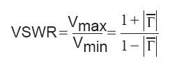
The numerical value of VSWR is in the range between 1 (ideally matched load, no standing wave) and ∞ (|Γ| = 1, total reflection or complete mismatch).

VSWR, Γ, RL, and ML describe the same phenomenon of reflection and can be transformed into each other. While VSWR and RL are related to the amplitude of the reflected wave only, Γ contains the phase information too, as Γ is a complex quantity.

Often the antenna has an impedance different from that of the feeding transmission line. To minimize the mismatch loss, we have to transform one impedance to the complex conjugate of the other. A powerful tool that helps to determine the needed matching circuit is the Smith Chart. Basically, the Smith Chart plots the reflection coefficient Γ in the complex plane. For passive circuits, the length of the Γ-phasor varies between 0 (ideal match) and 1 (complete mismatch). The phase difference f between the reflected and the incident wave may assume any value between 0 and 2π. Therefore, all possible Γ-phasors (for passive circuits) are within a circle with the radius 1, which defines the outer boundary of the Smith Chart.

The reflection coefficient is +1 if the end of a transmission line is left open, −1 for a short at the end of the transmission line. An inductive load gives a reflection coefficient in the upper half, a capacitive load in the lower half of the Smith Chart. Any capacitors or inductors added to a given load move the reflection coefficient in the Smith Chart on circles: series components on a circle that goes through the open point at +1, parallel components on circles through the shortcut point at −1. Inductors shift the reflection coefficient upwards towards the inductive half; capacitors shift it downwards towards the capacitive half. Figure 5 shows how series or parallel inductors and capacitors influence a given reflection coefficient.

Using the Smith Chart we can find out what kind of components are needed to minimize the reflection coefficient for a given antenna impedance. In Figure 5 for example, a series capacitor could move the reflection coefficient on the circle through the open point (because it is a series component) towards the lower half of the Smith Chart (because it is a capacitor). The center of the Smith Chart (where the reflection coefficient is zero) can be reached by a proper capacitance value giving the perfect match.

For a system environment normalized to 50 Ω, the center of the Smith Chart is 50 Ω.

Note: Image can view in larger size, if you open in a new tab